Use of Density-based Partial Routes

Imagine that in a bustling building, a train station for example, two pedestrians have two different paths available to them between two key points. One of the two paths can be seen for the most part, while the other has a larger section that is not initially visible (named as ‘concealed’ path).

It is obvious how people make the decision in real life: the actual density on the path that can be seen, will be compared with the supposed situation in the section that cannot be seen. This imagined situation may or may not be accurate. The real situation can vary in either direction – there may be a higher or lower density of people.

How can that be modelled in PTV Viswalk? For the partial routes of type “travel time”, which have already been part of the Viswalk functions for longer, only the actual measured travel time of each route is used as a basis for making decisions. For the dynamic potential too, “only” information regarding the actual situation is sent to the pedestrians who have to make a decision. Again, here the chosen path is related to the situation all along that path.

Since PTV Viswalk 7, it is possible to assign partial routing decisions based on the number of pedestrians or the density in areas as a basis for making decisions for individual partial routes. The areas assigned to a partial route do not have to be along this route, but may optionally be far from it – even so far that the situation on these areas can have no influence on the situation of the areas along the partial route. At first, it must appear nonsensical to assign areas so far from a partial route as the principle for the decision. This can, however, be utilized explicitly to model the supposed situation on the concealed path.

_{llustration 1} 

Sample model depicting the described situation diagrammatically. The left illustration shows the view from above, while the right one shows the same scene from the pedestrian’s point of view. The relevant pedestrian flow starts in the large green area on the left and needs to move to the red area. Additional pedestrians can be introduced into the model via both the smaller green areas, and these then also go towards the red area and therefore add to the density in the corridors. The orange obstacles depicted are high, while the blue ones are low (e.g. garden ponds). Because of this, before reaching the branch, the pedestrians have information on the situation in the lower corridor (to the right of the pedestrian’s view), but not for the upper corridor.

Illustration 1 depicts an extremely simplified model applying the idea described. On the way from the start to the destination, the pedestrians can choose between two alternative paths of comparable geometry (same length, same width). One of the two paths can be seen, while the other for the most part cannot.

To model the decision between both alternatives, a partial routing decision (method: density) is created in an additional area. From here, there are two routes to the destination (to the right): one of the routes has an intermediate destination on the right path, while the other on the left path (see Illustration 2).

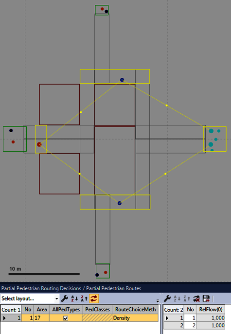
 _{Illustration 2: Partial routing decision and partial routes. You can access the displayed list via the menu Lists – Pedestrian traffic – Partial Routing decisions}

Now, for each of the two partial routes, those areas need to be selected, at which the pedestrian density is measured and used to calculate the route proportions. Illustration 3 shows this for the right path.

Illustration 3: You can open the list shown below by going to the menu Lists – Pedestrian traffic – Partial routes. Then choose as secondary list Pedestrian route choice areas. Right-click on the secondary list to create a new item. In the illustration the areas 3, 7 and 8 (i.e. the areas along the path) are assigned to that route that directs pedestrians along the areas 3, 7 and 8 (the right-hand path).

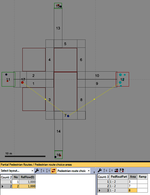
_{Illustration 3}

Technically speaking, it would now of course be possible to assign the areas 4, 5 and 6 (see Illustration 3) to the partial route along the left path. However, the modelled situation would then be as such as these areas can be seen by the pedestrians at the moment of their decision.

Instead, a copy is made of the concealed section, and a pedestrian input as well as a route is added. The input does not depict an actual event, but models how the pedestrians, who make their route choice, imagine the situation in the “invisible” section (see Illustration 4).

Illustration 4: Instead of the areas 5 and 6, the areas 18 and 19 are designated as decision areas for the left-hand path. In this example, area 4 is not replaced by another area because the very pedestrians making the decision can see how many pedestrians turn in front of them and therefore have an idea of the density of area 4.

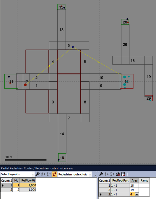
_{Illustration 4}

Now the parameters of the partial routing decision still need to be configured. This can be done in the list of the partial routing decisions. A more straightforward method is by editing the corresponding dialog (see Illustration 5).

Illustration 5: Configure the settings in the partial routing decision dialog for the Density method as follows: -Decision model: Entering the area: the pedestrians decide once, i.e. when entering the decision area (instead of at each time step while located in the area with the partial routing decision). -Pedestrian classes: All pedestrian types. -Route choice parameters: the route choice proportions are calculated from the density using the Logit function. The parameter used for this, 0.5 ped/m², is comparatively small and allows pedestrians to react quite sensitively to small changes in density. Useful values are around the density of the maximum specific flow (~1.3/m²) (factor 0.1 to 10). -Combination method: Average: for each path, the average of all three measured densities is used to calculate the total density of the path.

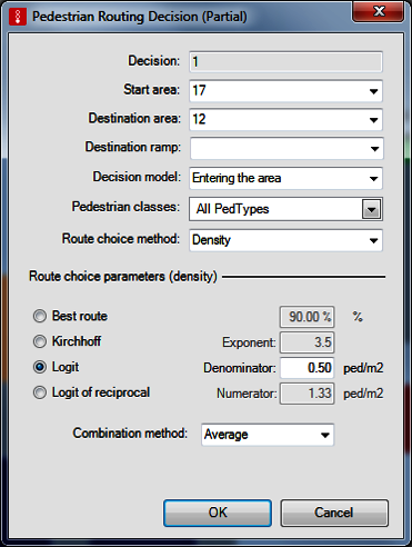
_{Illustration 5}

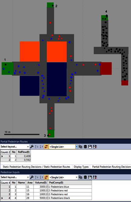
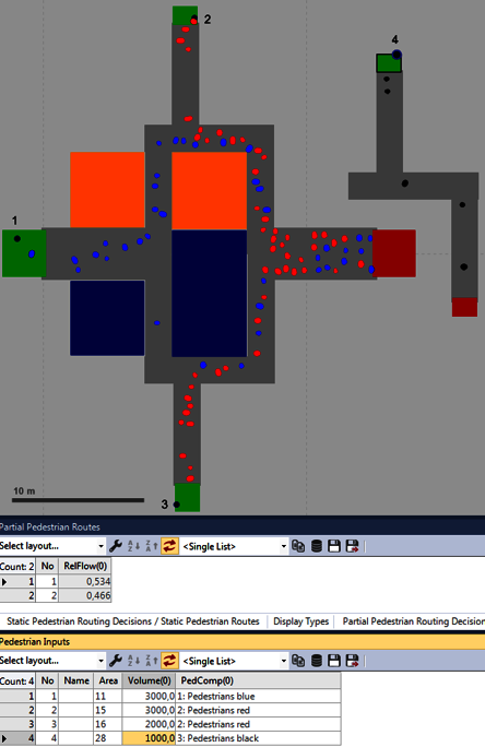
Illustration 6: The blue pedestrians considerably overestimate the density of the concealed part of the corridor. The majority therefore take the right-hand path. The list of partial routes shows the relevant latest route choice proportions. Illustration 7: Here the opposite happens to the previous illustration: the blue pedestrians underestimate the density in the concealed area. Therefore, too many pedestrians choose the left (upper) path.

Illustration 8: Here, finally the blue pedestrians make a correct assessment.

As an extension to this route choice method, combinations of different criteria can also be modelled, for example:

• different assessment abilities (commuters/tourists) and
• different character traits (optimist/pessimist

To do this, the concealed path area is repeatedly duplicated and, in accordance with the above criteria, different pedestrian demand is added. The pedestrians are then divided into several classes so that the partial routes (and their decisions) can be modelled differently for each pedestrian class.

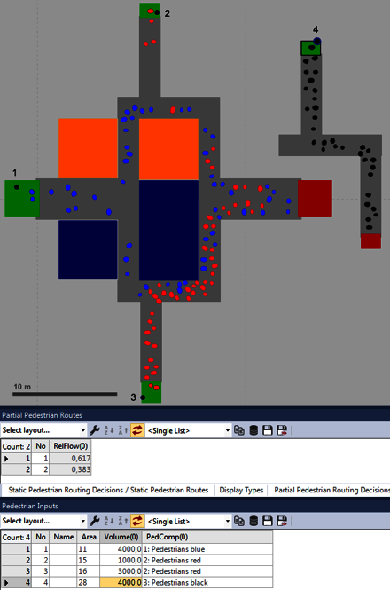
_{Illustration 8}